Generating a thermal evolution curve
Note
Download the full notebook : here
To obtain the internal temperature (or luminosity) and radius as a function of age, we need to use the GASTLI class Thermal_evolution. This class obtains a sequence of static interior-atmosphere models at different internal temperatures with the function thermal_evolution_class_object.main(). The input array Tint_array specifies the discreet internal temperatures at which the static models are computed. We recommend to save the sequence of interior models in a file, as in the example below. In this example, we name the thermal evolution class object my_therm_obj. The output of the main() thermal class function is:
The derivative of the entropy dS/dt in SI units:
thermal_evolution_class_object.f_SThe envelope entropy at 1000 bar in J/kg/K:
thermal_evolution_class_object.s_top_TEThe envelope mean entropy in J/kg/K:
thermal_evolution_class_object.s_mean_TEThe total planet radius, and interior radius (center to surface pressure) in Jupiter radii:
thermal_evolution_class_object.Rtot_TEandthermal_evolution_class_object.Rbulk_TEThe surface temperature in K:
thermal_evolution_class_object.Tsurf_TE
# Import GASTLI thermal module
import gastli.Thermal_evolution as therm
# Other Python modules
import numpy as np
# Create thermal evolution class object
my_therm_obj = therm.thermal_evolution()
# Input for interior
M_P = 18.76     # Earth units
# Equilibrium temperatures
Teqpl = 1000.
# Core mass fraction
CMF = 0.5
log_FeH = np.log10(20.) # 20 x solar
Tint_array = np.asarray([50.,60.,70.,80., 100., 110., 120., 130., 140., 160., 150., 160., 200., 240., 300.])
# Run sequence of interior models at different internal temperatures
my_therm_obj.main(M_P, CMF, Teqpl, Tint_array, log_FeH=log_FeH)
# Recommended: save sequence of interior models in case thermal evol eq. solver stops
Rjup = 11.2  # Jupiter radius in Earth units
data = np.zeros((len(my_therm_obj.f_S),7))
data[:,0] = my_therm_obj.f_S
data[:,1] = my_therm_obj.s_mean_TE
data[:,2] = my_therm_obj.s_top_TE
data[:,3] = my_therm_obj.Tint_array
data[:,4] = my_therm_obj.Rtot_TE*Rjup
data[:,5] = my_therm_obj.Rbulk_TE*Rjup
data[:,6] = my_therm_obj.Tsurf_TE
fmt = '%1.4e','%1.4e','%1.4e','%1.4e','%1.4e','%1.4e','%1.4e'
np.savetxt('thermal_sequence_HATP26b_CMF50_20xsolar.dat', data,header='f_S s_mean_TE s_top_TE Tint Rtot Rbulk    Tsurf',comments='',fmt=fmt)
Then this file can be read, and its columns are used to solve the luminosity differential equation by the function thermal_evolution_class_object.solve_thermal_evol_eq(). This function requires an age array in Gyr to solve the luminosity equation, t_Gyr. The default contains 100 points for fast computations, but for thermal evolution curves with ages younger than 1 Gyr, we recommend to use 10000 points, as in the example below. The final output is the corresponding radius array thermal_evolution_class_object.Rtot_solution. The array thermal_evolution_class_object.age_points contains the age evaluated at the static interior models.
# Import GASTLI thermal module
import gastli.Thermal_evolution as therm
# Other Python modules
import numpy as np
import matplotlib.pyplot as plt
from scipy import interpolate
import pandas as pd
# Create thermal evolution class
my_therm_obj = therm.thermal_evolution()
# Read in data saved in step 1
data = pd.read_csv('thermal_sequence_HATP26b_CMF50_20xsolar.dat', sep='\s+',header=None,skiprows=1)
my_therm_obj.f_S = data[0]
my_therm_obj.s_mean_TE = data[1]
my_therm_obj.s_top_TE = data[2]
my_therm_obj.Tint_array = data[3]
my_therm_obj.Rtot_TE = data[4]
my_therm_obj.Rbulk_TE = data[5]
my_therm_obj.Tsurf_TE = data[6]
my_therm_obj.solve_thermal_evol_eq(t_Gyr=np.linspace(2.1e-6, 15., 10000))
# Plot thermal evolution
fig = plt.figure(figsize=(6, 6))
ax = fig.add_subplot(1, 1, 1)
plt.title(r"Envelope composition: 20 $\times$ solar")
plt.plot(my_therm_obj.t_Gyr, my_therm_obj.Rtot_solution, '-', color='springgreen', linewidth=4.) #,label="CMF = 0.9")
plt.plot(my_therm_obj.age_points, my_therm_obj.Rtot_TE, 'o', color='springgreen', markeredgecolor='k')
plt.text(12.3,6.3,"CMF = 0.5")
# HAT-P-26 b radius and age data
yerr = np.zeros((2,1))
yerr[0,0] = 0.36
yerr[1,0] = 0.81
xerr = np.zeros((2,1))
xerr[0,0] = 4.9
xerr[1,0] = 3.
plt.errorbar([9.],[6.33], yerr, xerr,'X',color='black',label="HAT-P-26 b")
plt.legend()
plt.ylabel(r'Radius [$R_{\oplus}$]', fontsize=14)
plt.xlabel(r'Age [Gyrs]', fontsize=14)
plt.xlim(0.,15.)
plt.ylim(3.,10.)
# Save figure
fig.savefig('thermal_evolution_HATP26b_20xsolar.pdf', bbox_inches='tight', format='pdf', dpi=1000)
plt.close(fig)
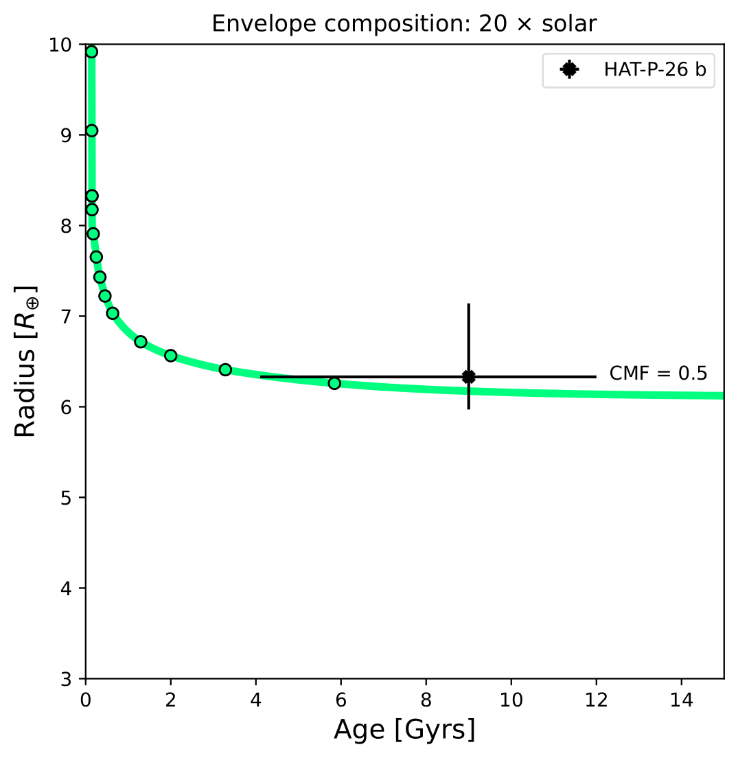
Radius evolution of HAT-P-26 b for CMF = 0.5 and 20 x solar envelope composition.
The output arrays thermal_evolution_class_object.Tint_solution and thermal_evolution_class_object.S_solution can be used to plot the internal temperature and luminosity, and the entropy, respectively:
# Plot thermal evolution
fig = plt.figure(figsize=(19, 6))
# Entropy
ax = fig.add_subplot(1, 3, 1)
plt.plot(my_therm_obj.t_Gyr, my_therm_obj.S_solution/1e6, linestyle='solid', color='black',linewidth=4)
plt.plot(my_therm_obj.age_points, my_therm_obj.s_top_TE/1e6, 'o', color='grey', markeredgecolor='k')
plt.ylabel(r'Entropy [MJ/kg/K]', fontsize=14)
plt.xlabel(r'Age [Gyrs]', fontsize=14)
ax.set_xscale('log')
plt.xlim(1e-2,12.)
plt.ylim(0.03,0.12)
plt.legend()
# Internal (or intrinsic) temperature
ax = fig.add_subplot(1, 3, 2)
plt.plot(my_therm_obj.t_Gyr, my_therm_obj.Tint_solution, linestyle='solid', color='black',linewidth=4)
plt.plot(my_therm_obj.age_points, my_therm_obj.Tint_array, 'o', color='grey', markeredgecolor='k')
plt.ylabel(r'T$_{int}$ [K]', fontsize=14)
plt.xlabel(r'Age [Gyrs]', fontsize=14)
ax.set_xscale('log')
plt.xlim(1e-2,12.)
plt.ylim(0.,1000)
# Luminosity
ax = fig.add_subplot(1, 3, 3)
sigma = 5.67e-8
Lsun = 3.846e26
Lint = (4 * np.pi * sigma * (my_therm_obj.Rtot_TE*11.2*cte.constants.r_e)**2 * my_therm_obj.Tint_array**4)/Lsun
Lsolution = (4 * np.pi * sigma * (my_therm_obj.Rtot_solution*11.2*cte.constants.r_e)**2 *\
          my_therm_obj.Tint_solution**4)/Lsun
plt.plot(my_therm_obj.t_Gyr, Lsolution, linestyle='solid', color='black',linewidth=4)
plt.plot(my_therm_obj.age_points, Lint, 'o', color='grey', markeredgecolor='k')
plt.ylabel(r'Luminosity [L$_{sun}$]', fontsize=14)
plt.xlabel(r'Age [Gyrs]', fontsize=14)
ax.set_yscale('log')
ax.set_xscale('log')
plt.xlim(1e-2,12.)
# Save plot
fig.savefig('thermal_evolution_all.pdf', bbox_inches='tight', format='pdf', dpi=1000)
plt.close(fig)
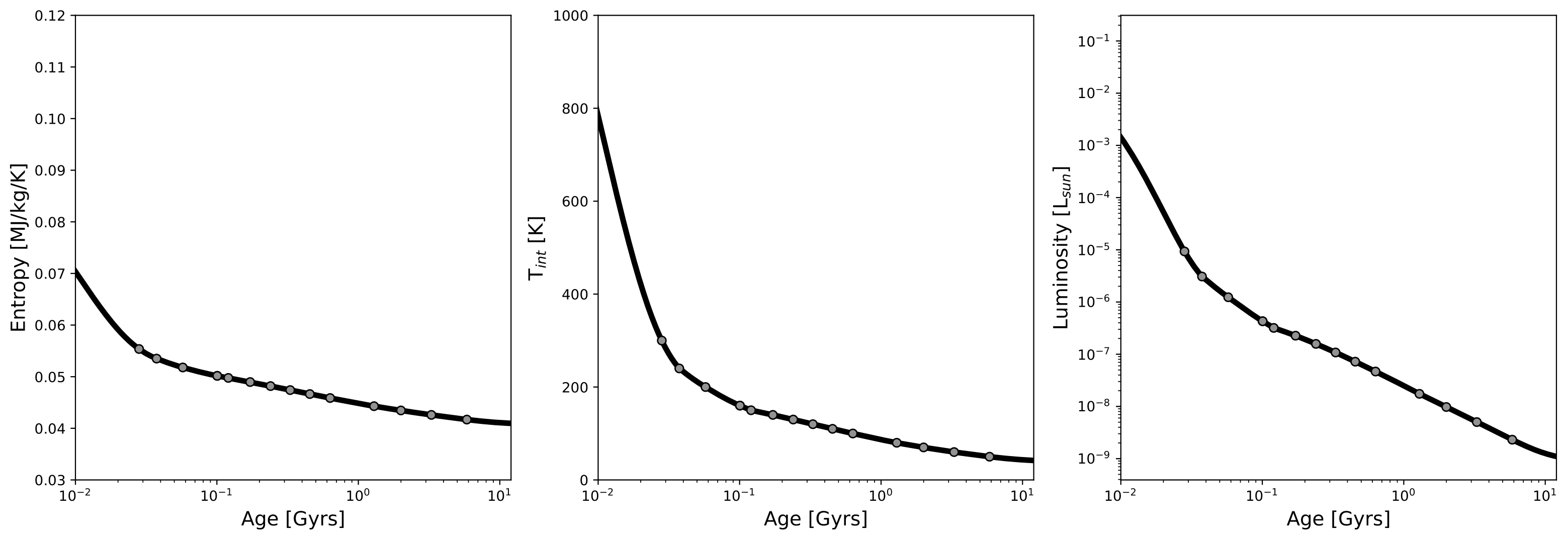
Entropy, internal temperature, and luminosity of HAT-P-26 b for CMF = 0.5 and 20 x solar envelope composition.