Interior retrievals
Note
Download the full notebook : here
In this page we show a tutorial on how to obtain a grid of GASTLI models to run a retrieval on mass, radius, age, and atmospheric metallicity.
We first need to generate a grid of forward models. The next example is going to consist of more than 4000 models. Each model takes between 2-10 second, so this may take up to 12 hours, depending on the computer architecture and number of threads/cores available for parallelization. Hence, we recommend setting up this step of the calculation in a cluster. The following code saves each thermal evolution curve in a file:
# Import coupling module
import gastli.Thermal_evolution as therm
# Other Python modules
import numpy as np
import os

Mjup = 318.
Rjup = 11.2
## Equilibrium temperature
Teqpl = 842.
# Input for interior
## mass in Mearth units
mass = np.arange(0.4*Mjup,1.05*Mjup,0.05*Mjup)
## CMF
CMFs = np.array([0.,0.1,0.2,0.25,0.3,0.35,0.4,0.45,0.5,0.6,0.8,0.99])
## log(Fe/H)
log_FeHs = np.array([-2.,0.,1.,1.99])
## Tint
Tint_array = np.array([50.,100.,200.,300.,400.,449.])
# Loop for forward models
n_mrel = len(CMFs)*len(log_FeHs)*len(mass)
counter = 0
for i_cmf, CMF in enumerate(CMFs):
    for i_FeH, logFeH in enumerate(log_FeHs):
        for i_mass, M_P in enumerate(mass):
            counter = counter+1
            # File with thermal evolution
            file_name = "Output/thermal_sequence_CMF_" + "{:4.2f}".format(CMF) + "_logFeH_" + "{:4.2f}".format(logFeH) +\
                      "_mass_" + "{:4.2f}".format(M_P) + ".dat"
            # Check that file does not exist to avoid overwrite
            answer = os.path.isfile(file_name)
            if answer == True:
               continue
           # Print message to monitor progress
           print('---------------')
           print('CMF = ', CMF)
           print('log(Fe/H) = ', logFeH)
           print('Mass [Mearth] = ', M_P)
           print('Sequence = ', counter, ' out of ', n_mrel)
           print('---------------')
           # Thermal evolution class object
           my_therm_obj = therm.thermal_evolution(pow_law_formass=0.315)
           my_therm_obj.main(M_P, CMF, Teqpl, Tint_array, CO=0.55, log_FeH=logFeH)
           my_therm_obj.solve_thermal_evol_eq()
           # Save sequence of interior models
           data = np.zeros((len(my_therm_obj.f_S), 11))
           data[:, 0] = my_therm_obj.f_S
           data[:, 1] = my_therm_obj.s_mean_TE
           data[:, 2] = my_therm_obj.s_top_TE
           data[:, 3] = my_therm_obj.Tint_array
           data[:, 4] = my_therm_obj.Rtot_TE*Rjup
           data[:, 5] = my_therm_obj.Rbulk_TE*Rjup
           data[:, 6] = my_therm_obj.Tsurf_TE
           data[:, 7] = my_therm_obj.age_points
           data[:, 8] = my_therm_obj.Zenv_TE
           data[:, 9] = my_therm_obj.Mtot_TE
           tmm = CMF + (1-CMF)*my_therm_obj.Zenv_TE
           data[:, 10] = tmm
           header0 = 'f_S s_mean_TE s_top_TE Tint_K Rtot_earth Rbulk_earth Tsurf_K Age_Gyrs Zenv Mtot_earth Zplanet'
           np.savetxt(file_name, data, header=header0, comments='',fmt = '%1.4e')
Then, we can read all these files in a loop to generate a single hdf5 grid with all the forward models:
# Python modules
import numpy as np
import pandas as pd
import h5py
# Constants
Mjup = 318.
Rjup = 11.2
# Arrays of grid
## mass in Mearth units
masses = np.arange(0.4*Mjup,1.05*Mjup,0.05*Mjup)
## CMF
CMFs = np.array([0.,0.1,0.2,0.25,0.3,0.35,0.4,0.45,0.5,0.6,0.8,0.99])
## log(Fe/H)
log_FeHs = np.array([-2.,0.,1.,1.99])
## Tint
Tint_array = np.array([50.,100.,200.,300.,349.])
n_masses  = len(masses)
n_logFeH = len(log_FeHs)
n_CMF= len(CMFs)
n_Tint = len(Tint_array)
# Create file
f = h5py.File("my_forward_model_grid.hdf5", "w")
# Data sets
data_set_Rtot = f.create_dataset("Rtot", (n_CMF, n_logFeH, n_masses, n_Tint), dtype='f')
data_set_Rbulk = f.create_dataset("Rbulk", (n_CMF, n_logFeH, n_masses, n_Tint), dtype='f')
data_set_age = f.create_dataset("age", (n_CMF, n_logFeH, n_masses, n_Tint), dtype='f')
data_set_Tsurf = f.create_dataset("Tsurf", (n_CMF, n_logFeH, n_masses, n_Tint), dtype='f')
data_set_Mtot = f.create_dataset("Mtot", (n_CMF, n_logFeH, n_masses, n_Tint), dtype='f')
data_set_Zplanet = f.create_dataset("Zplanet", (n_CMF, n_logFeH, n_masses, n_Tint), dtype='f')
data_set_Zenv = f.create_dataset("Zenv", (n_CMF, n_logFeH, n_masses, n_Tint), dtype='f')
# Assign arrays for grid
f['CMF'] = CMFs
f['log_FeH'] = log_FeHs
f['mass'] = masses/Mjup
f['Tint'] = Tint_array
# Prepare loop to read output files and fill in data sets
n_mrel = n_CMF*n_logFeH*n_masses
for i_cmf, CMF in enumerate(CMFs):
    for i_FeH, logFeH in enumerate(log_FeHs):
        for i_mass, M_P in enumerate(masses):
            file_name = "Output/thermal_sequence_CMF_" + "{:4.2f}".format(CMF) +\
                     "_logFeH_" + "{:4.2f}".format(logFeH) + "_mass_" + "{:4.2f}".format(M_P) + ".dat"
            # Read file
            data = pd.read_csv(file_name, sep='\s+', header=0)
            rtot = data['Rtot_earth']
            rbulk = data['Rbulk_earth']
            age = data['Age_Gyrs']
            tsurf = data['Tsurf_K']
            mtot = data['Mtot_earth']
            zplanet = data['Zplanet']
            zenv = data['Zenv']
            # Fill data set
            data_set_Rtot[i_cmf, i_FeH, i_mass, :] = rtot/Rjup
            data_set_Rbulk[i_cmf, i_FeH, i_mass, :] = rbulk/Rjup
            data_set_age[i_cmf, i_FeH, i_mass, :] = age
            data_set_Tsurf[i_cmf, i_FeH, i_mass, :] = tsurf
            data_set_Mtot[i_cmf, i_FeH, i_mass, :] = mtot/Mjup
            data_set_Zplanet[i_cmf, i_FeH, i_mass, :] = zplanet
            data_set_Zenv[i_cmf, i_FeH, i_mass, :] = zenv
# End of loop, now attach dimensions to grid data sets
## Total radius (Jupiter units)
f['Rtot'].dims[0].attach_scale(f['CMF'])
f['Rtot'].dims[1].attach_scale(f['log_FeH'])
f['Rtot'].dims[2].attach_scale(f['mass'])
f['Rtot'].dims[3].attach_scale(f['Tint'])
## Interior radius
f['Rbulk'].dims[0].attach_scale(f['CMF'])
f['Rbulk'].dims[1].attach_scale(f['log_FeH'])
f['Rbulk'].dims[2].attach_scale(f['mass'])
f['Rbulk'].dims[3].attach_scale(f['Tint'])
## Age (Gyrs)
f['age'].dims[0].attach_scale(f['CMF'])
f['age'].dims[1].attach_scale(f['log_FeH'])
f['age'].dims[2].attach_scale(f['mass'])
f['age'].dims[3].attach_scale(f['Tint'])
## Surface temperature (K)
f['Tsurf'].dims[0].attach_scale(f['CMF'])
f['Tsurf'].dims[1].attach_scale(f['log_FeH'])
f['Tsurf'].dims[2].attach_scale(f['mass'])
f['Tsurf'].dims[3].attach_scale(f['Tint'])
## Total mass (Jupiter units)
f['Mtot'].dims[0].attach_scale(f['CMF'])
f['Mtot'].dims[1].attach_scale(f['log_FeH'])
f['Mtot'].dims[2].attach_scale(f['mass'])
f['Mtot'].dims[3].attach_scale(f['Tint'])
## Total metal mass fraction
f['Zplanet'].dims[0].attach_scale(f['CMF'])
f['Zplanet'].dims[1].attach_scale(f['log_FeH'])
f['Zplanet'].dims[2].attach_scale(f['mass'])
f['Zplanet'].dims[3].attach_scale(f['Tint'])
## Envelope metal mass fraction
f['Zenv'].dims[0].attach_scale(f['CMF'])
f['Zenv'].dims[1].attach_scale(f['log_FeH'])
f['Zenv'].dims[2].attach_scale(f['mass'])
f['Zenv'].dims[3].attach_scale(f['Tint'])
# Close file
f.close()
We finally have our grid of forward models that we can interpolate. For the retrieval, you need to install the Markov chain Monte Carlo (MCMC) sampler package emcee. The following snippet uses emcee and interpolates our grid to perform the retrieval.
# import modules
import numpy as np
import h5py
from scipy.interpolate import RegularGridInterpolator
import matplotlib.pyplot as plt
import emcee
# Load data
file_name = "my_forward_model_grid.hdf5"
file = h5py.File(file_name, 'r')
## datasets
data_set_Rtot = file['Rtot'][()]
data_set_Rbulk = file['Rbulk'][()]
data_set_age = file['age'][()]
data_set_Tsurf = file['Tsurf'][()]
data_set_Mtot = file['Mtot'][()]
data_set_Zplanet = file['Zplanet'][()]
data_set_Zenv = file['Zenv'][()]
## arrays
CMFs = file['CMF'][()]
logFeHs = file['log_FeH'][()]
masses = file['mass'][()]
Tints = file['Tint'][()]
# Create functions for interpolation
rtot = RegularGridInterpolator((CMFs,logFeHs,masses,Tints), data_set_Rtot, bounds_error=False, fill_value=None)
rbulk = RegularGridInterpolator((CMFs,logFeHs,masses,Tints), data_set_Rbulk, bounds_error=False, fill_value=None)
age = RegularGridInterpolator((CMFs,logFeHs,masses,Tints), data_set_age, bounds_error=False, fill_value=None)
tsurf = RegularGridInterpolator((CMFs,logFeHs,masses,Tints), data_set_Tsurf, bounds_error=False, fill_value=None)
mtot = RegularGridInterpolator((CMFs,logFeHs,masses,Tints), data_set_Mtot, bounds_error=False, fill_value=None)
zplanet = RegularGridInterpolator((CMFs,logFeHs,masses,Tints), data_set_Zplanet, bounds_error=False, fill_value=None)
zenv = RegularGridInterpolator((CMFs,logFeHs,masses,Tints), data_set_Zenv, bounds_error=False, fill_value=None)
# Forward model function
def forward_model(CMF, logFeH, bulk_mass, Tint_mod):
    '''
    Forward model
    '''
    pts = np.zeros((1, 4))
    pts[:, 0] = CMF
    pts[:, 1] = logFeH
    pts[:, 2] = bulk_mass
    pts[:, 3] = Tint_mod
    model_R = rtot(pts)
    R_mod = model_R[0]
    model_Mtot = mtot(pts)
    Mtot_mod = model_Mtot[0]
    model_age = age(pts)
    age_mod = model_age[0]
    return R_mod, Mtot_mod, age_mod
# Example of use
output_forward = forward_model(0.1, 0., 0.74, 70.)
print(output_forward)
# Log-likelihood
## Mass, radius and age: mean and uncertainties
mean_mass = 0.74
e_M_minus = 0.07
e_M_plus = 0.06
age_planet = 7.3
e_age_minus = 2.5
e_age_plus = 2.4
mean_rad = 0.98
e_rad_minus = 0.05
e_rad_plus = 0.05
x = np.asarray([])
y = np.asarray([mean_mass,mean_rad,age_planet])
yerr = np.asarray([e_M_plus,e_M_minus,e_rad_plus,e_rad_minus,e_age_plus,e_age_minus])
'''
Format:
y = (Mp,Rp,age)
yerr = (Mp_e+,Mp_e-,Rp_e+,Rp_e-,age_e+,age_e-)
'''
## Function
def log_likelihood(theta, x, y, yerr):
    CMF_mod, log_FeH_mod, mass_mod, Tint_mod = theta
    R_mod, Mtot_mod, age_mod  = forward_model(CMF_mod, log_FeH_mod, mass_mod, Tint_mod)
    Mdata = y[0]
    Rdata = y[1]
    age_data = y[2]
    sigma_Mplus = yerr[0]
    sigma_Mminus = yerr[1]
    sigma_Rplus = yerr[2]
    sigma_Rminus = yerr[3]
    sigma_age_plus = yerr[4]
    sigma_age_minus = yerr[5]
    if Mtot_mod > Mdata:
       sigma_M = sigma_Mplus
    else:
       sigma_M = sigma_Mminus
    if R_mod > Rdata:
       sigma_R = sigma_Rplus
    else:
       sigma_R = sigma_Rminus
    if age_mod > age_data:
       sigma_age = sigma_age_plus
    else:
       sigma_age = sigma_age_minus
    # Likelihood
    L = -0.5 * ( ((Mtot_mod - Mdata) / sigma_M) ** 2 + \
              ((R_mod - Rdata) / sigma_R) ** 2+\
              ((age_mod - age_planet) / sigma_age)**2 )
    return L
# Example of use
theta_test = np.array([0.1, 0., 0.74, 70.])
a = log_likelihood(theta_test, x, y, yerr)
print(a)
# Priors
## Max and min limits
CMF_min = 0.01
CMF_max = 0.99
logFeH_min = -2.
logFeH_max = 1.99
mass_min = 0.4
mass_max = 1.05
Tint_min = 50.
Tint_max = 349.
# Function
def log_prior(theta):
    CMF_mod, log_FeH_mod, mass_mod, Tint_mod = theta
    if min(CMFs) < CMF_mod < max(CMFs) and \
    min(logFeHs) < log_FeH_mod < max(logFeHs) and \
    min(masses) < mass_mod < max(masses) and \
    Tint_min < Tint_mod < Tint_max:
        return 0.0
    return -np.inf
 # Probability function
 def log_probability(theta, x, y, yerr):
     lp = log_prior(theta)
     if not np.isfinite(lp):
        return -np.inf
     return lp + log_likelihood(theta, x, y, yerr)
 # Define walkers
 nwlk = 32
 pos = np.zeros((nwlk, 4))
 pos[:,0] = np.random.uniform(CMF_min, CMF_max, nwlk)                   # CMF: uniform
 pos[:,1] = np.random.uniform(logFeH_min, logFeH_max, nwlk)             # log(Fe/H): uniform
 pos[:,2] = np.random.normal(mean_mass, max(e_M_plus,e_M_minus), nwlk)  # mass: uniform
 pos[:,3] = np.random.uniform(Tint_min, Tint_max, nwlk)                 # Tint: log-uniform
 nwalkers, ndim = pos.shape
 # Define steps
 nsteps = int(100000)
 # emcee main functions
 sampler = emcee.EnsembleSampler(
 nwalkers, ndim, log_probability, args=(x, y, yerr), backend=backend
 )
 sampler.run_mcmc(pos, nsteps, progress=True)
A retrieval with this number of steps takes around 30 min. To check convergence, we can plot the evolution of the chains:
fig, axes = plt.subplots(ndim, figsize=(10, 11), sharex=True)
samples = sampler.get_chain()
labels = ["CMF", "log(FeH) [x solar]", "Mass [MJup]", "Tint [K]"]
for i in range(ndim):
    ax = axes[i]
    ax.plot(samples[:, :, i], "k", alpha=0.3)
    ax.set_xlim(0, len(samples))
    ax.set_ylabel(labels[i])
    ax.yaxis.set_label_coords(-0.1, 0.5)
axes[-1].set_xlabel("step number")
fig.savefig('Output/emcee_convergence.pdf',bbox_inches='tight',format='pdf', dpi=1000)
plt.close(fig)
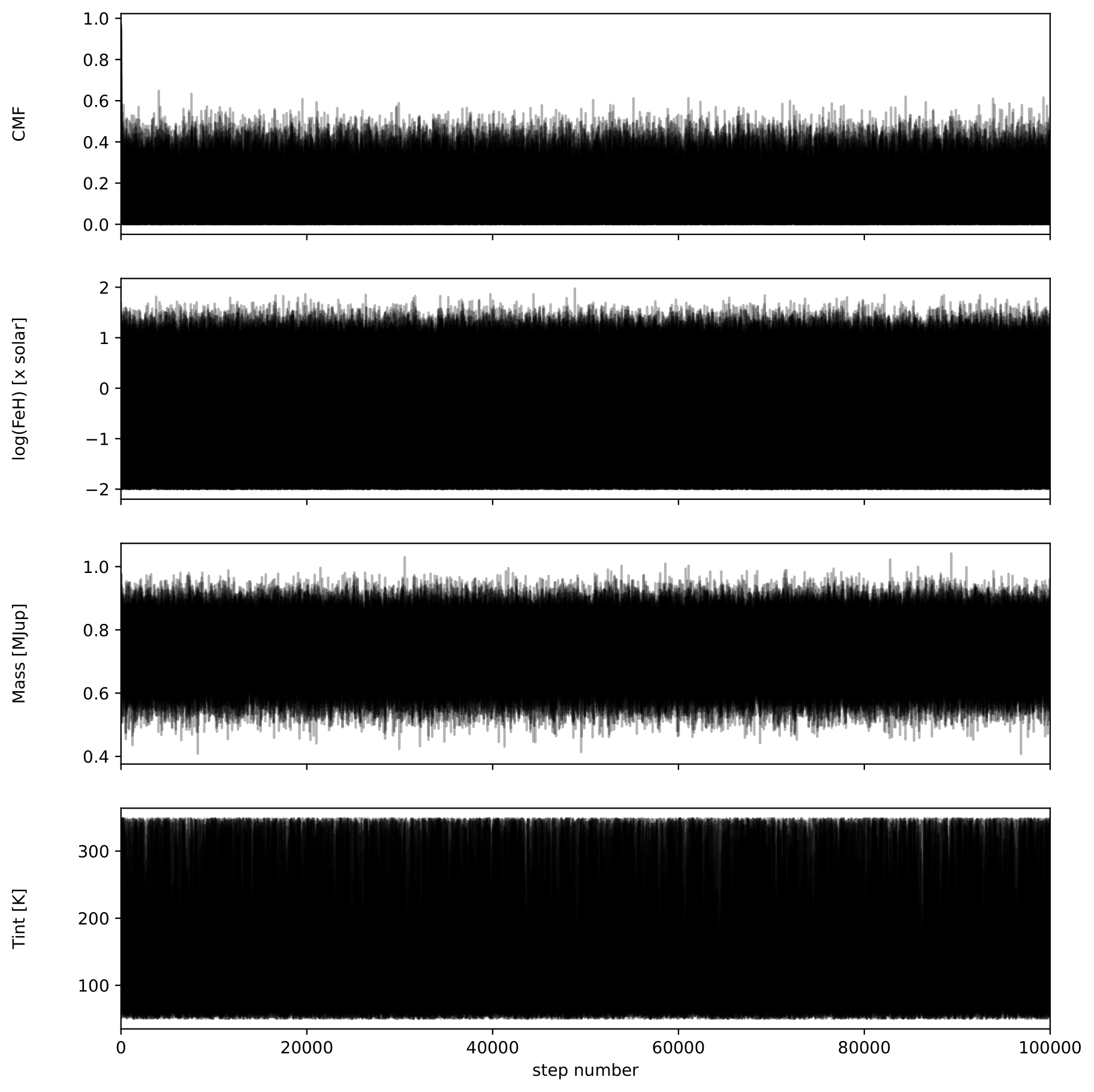
You can also check that the MCMC chains converged by looking at the autocorrelation time
tau = sampler.get_autocorr_time()
print('tau = ', tau)
The autocorrelation time should not be larger than the number of steps divided by 50.
We can obtain the samples and save them with:
# Obtain input parameter samples
ndiscard = int(2 * max(tau))
nthin = int(max(tau)/2)
flat_samples = sampler.get_chain(discard=ndiscard, thin=nthin, flat=True)
n = flat_samples.shape[0]
CMF_sample = flat_samples[:, 0]
logFeH_sample = flat_samples[:, 1]
mass_sample = flat_samples[:, 2]
tint_sample = flat_samples[:, 3]
# Output parameter
## Initialise arrays
rtot_sample = np.zeros_like(CMF_sample)
mtot_sample = np.zeros_like(CMF_sample)
rbulk_sample = np.zeros_like(CMF_sample)
age_sample = np.zeros_like(CMF_sample)
tsurf_sample = np.zeros_like(CMF_sample)
zplanet_sample = np.zeros_like(CMF_sample)
zenv_sample = np.zeros_like(CMF_sample)
## Interpolate
pts = np.zeros((n, 4))
pts[:, 0] = CMF_sample
pts[:, 1] = logFeH_sample
pts[:, 2] = mass_sample
pts[:, 3] = tint_sample
rtot_sample = rtot(pts)
mtot_sample = mtot(pts)
rbulk_sample = rbulk(pts)
age_sample = age(pts)
tsurf_sample = tsurf(pts)
zplanet_sample = zplanet(pts)
zenv_sample = zenv(pts)
# Save all samples in output file
data = np.zeros((n,11))
data[:,0] = CMF_sample
data[:,1] = logFeH_sample
data[:,2] = mass_sample
data[:,3] = age_sample
data[:,4] = rtot_sample
data[:,5] = mtot_sample
data[:,6] = rbulk_sample
data[:,7] = tint_sample
data[:,8] = tsurf_sample
data[:,9] = zplanet_sample
data[:,10] = zenv_sample
np.savetxt('samples.dat', data,\
        header='CMF logFeH Mbulk[M_J] Age[Gyr] Rtot[R_J] Mtot[M_J] Rbulk[R_J] Tint[K] Tsurf[K] Zpl Zenv',\
        comments='',fmt='%1.4e')
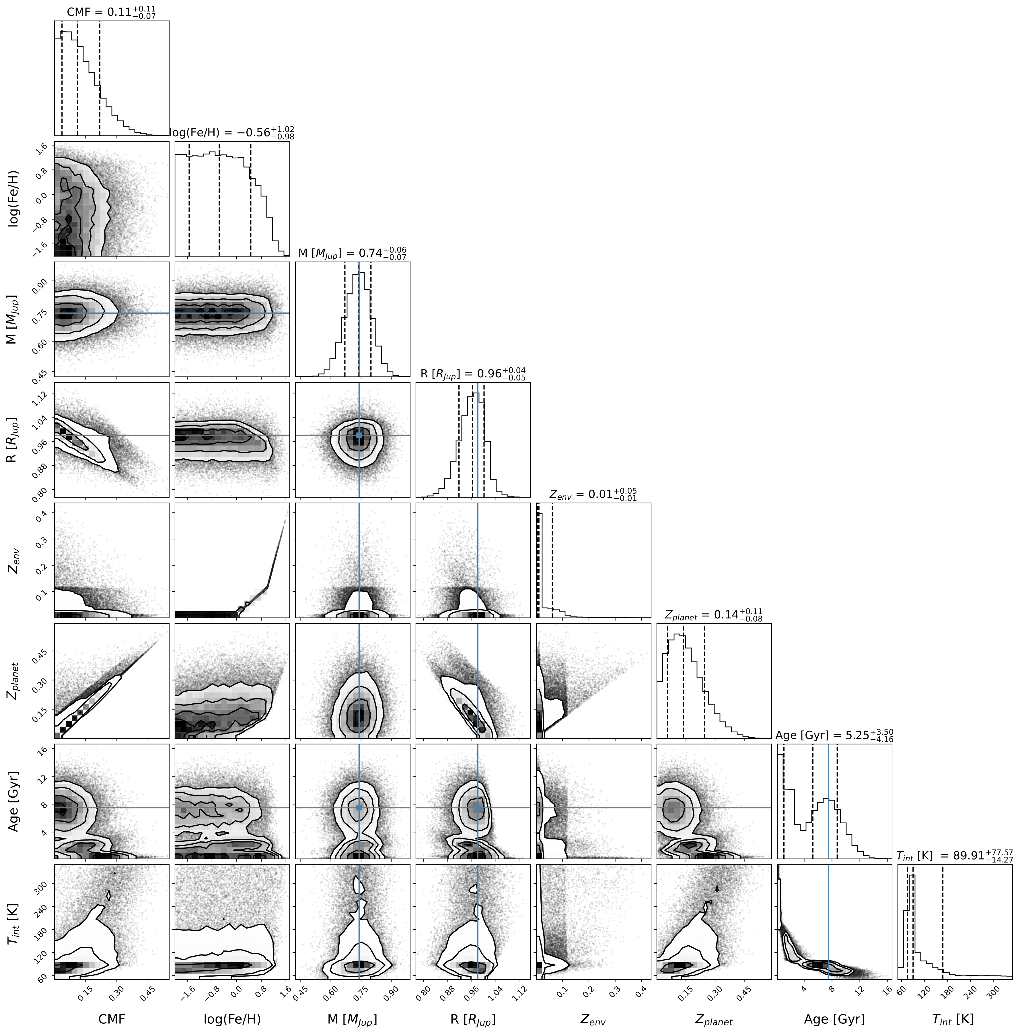
Finally, we can generate a corner plot with the samples with the module corner (see how to install it here). Here is a snippet to plot the samples obtained above:
# python modules
import pandas as pd
import numpy as np
import corner
# Read samples file
data = pd.read_csv('samples.dat', sep='\s+')
CMF = data['CMF']
log_FeH = data['logFeH']
M = data['Mtot[M_J]']
R = data['Rtot[R_J]']
Mbulk = data['Mbulk[M_J]']
Zenv = data['Zenv']
age = data['Age[Gyr]']
Tint = data['Tint[K]']
# Account for atmospheric mass (this is usually negligible)
Matm = M - Mbulk
Menv_int = Mbulk * (1-CMF)
EMF_recalc = (Menv_int + Matm)/M
x_core = 1. - EMF_recalc
Zplanet = x_core + EMF_recalc*Zenv
# Corner input
flat_samples = np.zeros((len(CMF),8))
flat_samples[:,0] = CMF
flat_samples[:,1] = log_FeH
flat_samples[:,2] = M
flat_samples[:,3] = R
flat_samples[:,4] = Zenv
flat_samples[:,5] = Zplanet
flat_samples[:,6] = age
flat_samples[:,7] = Tint
# Plot it.
figure = corner.corner(flat_samples, labels=[r"CMF", r"log(Fe/H)", r"M [$M_{Jup}$]",\
                                          r"R [$R_{Jup}$]", "$Z_{env}$", r"$Z_{planet}$", r"Age [Gyr]",\
                                          r"$T_{int}$ [K] "],
                    quantiles=[0.16, 0.5, 0.84],\
                    truths=[np.nan,np.nan,0.74,0.98,np.nan,np.nan,7.5,np.nan],\
                    show_titles=True, title_kwargs={"fontsize": 14},label_kwargs={"fontsize": 16})
figure.savefig('corner_plot.pdf',bbox_inches='tight',format='pdf', dpi=1000)