Creating an interior-atmosphere object
Note
Download the full notebook : here
You can start a simple interior-atmosphere object to generate one model by initialising the coupling class:
# Import coupling module
import gastli.Coupling as cpl
# Other Python modules
import numpy as np
# Initialise coupling class
my_coupling = cpl.coupling()
Next, specify the input variables for the interior-atmosphere model:
# Input for interior
# 1 Mjup in Mearth units
M_P = 318.
# Internal temperature
Tintpl = 99.
# Equilibrium temperature
Teqpl = 122.
# Core mass fraction
CMF = 0.01
If the log-metallicity of the atmosphere, \(log(Fe/H)\), is known, you must specify it as:
# Envelope log-metallicity is solar
log_FeHpl = 0
# C/O ratio is solar
CO_planet = 0.55
# Run coupled interior-atmosphere model
my_coupling.main(M_P, CMF, Teqpl, Tintpl, CO=CO_planet, log_FeH=log_FeHpl)
In a nutshell, you can print the output radius, total metal content, surface gravity, etc:
print("Case 1, log(Fe/H) is known")
# Composition input
print("log(Fe/H) atm [x solar] (input) = ",my_coupling.myatmmodel.log_FeH)
print("C/O atm (input) = ",my_coupling.myatmmodel.CO)
# Output
print("Zenv (output) = ",my_coupling.myatmmodel.Zenv_pl)
print("Total planet mass M [M_earth] = ",my_coupling.Mtot)
print("Temperature at 1000 bar [K] = ",my_coupling.T_surf)
print("Planet bulk radius [R_jup] = ",my_coupling.Rbulk_Rjup)
print("log10_g: Planet surface gravity (1000 bar) [cm/s2] = ",np.log10(my_coupling.g_surf_planet))
print("Total planet radius [R_jup] = ",my_coupling.Rtot)
tmm = my_coupling.Mtot*CMF + my_coupling.Mtot*(1-CMF)*my_coupling.myatmmodel.Zenv_pl
print("Total metal mass [M_earth] = ",tmm)
You will obtain the following output:
Case 1, log(Fe/H) is known
log(Fe/H) atm [x solar] (input) =  0
C/O atm (input) =  0.55
Zenv (output) =  0.013532983488449907
Total planet mass M [M_earth] =  318.0389824070297
Temperature at 1000 bar [K] =  1321.0792698333128
Planet bulk radius [R_jup] =  0.9732321589894197
log10_g: Planet surface gravity (1000 bar) [cm/s2] =  3.417144909504209
Total planet radius [R_jup] =  0.9795696861509946
Total metal mass [M_earth] =  7.441365958692064
On the other hand, if the envelope metal mass fraction is known instead of the log-metallicity, \(Z_{env}\), the flag FeH_flag=False must be used:
# Envelope metal mass fraction
Zenvpl = 0.013
# Run coupled interior-atmosphere model
my_coupling.main(M_P, CMF, Teqpl, Tintpl, FeH_flag=False, CO=CO_planet, Zenv=Zenvpl)
With its respective output summary:
Zenv (input) =  0.013
C/O atm (input) =  0.55
log(Fe/H) atm [x solar] (output) =  0.3130236027986046
Total planet mass M [M_earth] =  318.0393440504418
Temperature at 1000 bar [K] =  1358.2228909481744
Planet bulk radius [R_jup] =  0.9754815399424
log10_g: Planet surface gravity (1000 bar) [cm/s2] =  3.4151397013097373
Total planet radius [R_jup] =  0.9821050130682911
Total metal mass [M_earth] =  7.273559798433604
Interior structure profiles
To plot the interior structure profiles, we can obtain the arrays from the interior-atmosphere coupling class as:
Gravity in m/s 2:
coupling_class_object.myplanet.gPressure in Pa:
coupling_class_object.myplanet.PTemperature in K:
coupling_class_object.myplanet.TDensity in kg/m 3:
coupling_class_object.myplanet.rhoEntropy in J/kg/K:
coupling_class_object.myplanet.entropyRadius in m:
coupling_class_object.myplanet.r
Following the Jupiter example above (case 1, when the log-metallicity is known), the coupling class object was named my_coupling. We would add the following code to plot the 5 interior profiles as a function of radius:
# more modules
import gastli.constants as cte
import matplotlib.pyplot as plt
# Jupiter radius in Earth radii
Rjup_Rearth = 11.2
xmax = Rjup_Rearth*my_coupling.Rbulk_Rjup
# Plot interior profiles
fig = plt.figure(figsize=(6, 30))
# Panel 1: gravity
ax = fig.add_subplot(5, 1, 1)
plt.plot(my_coupling.myplanet.r / cte.constants.r_e, my_coupling.myplanet.g, '-', color='lime')
plt.xlabel(r'Radius [$R_{\oplus}$]', fontsize=16)
plt.ylabel(r'Gravity acceleration [$m/s^{2}$]', fontsize=16)
plt.xlim(0, xmax)
plt.ylim(0, 1.1 * np.nanmax(my_coupling.myplanet.g))
# Panel 2: pressure
ax = fig.add_subplot(5, 1, 2)
plt.plot(my_coupling.myplanet.r / cte.constants.r_e, my_coupling.myplanet.P / 1e9, '-', color='blue')
plt.xlabel(r'Radius [$R_{\oplus}$]', fontsize=16)
plt.ylabel('Pressure [GPa]', fontsize=16)
plt.xlim(0, xmax)
plt.ylim(0, 1.1 * np.amax(my_coupling.myplanet.P / 1e9))
# Panel 3: temperature
ax = fig.add_subplot(5, 1, 3)
plt.plot(my_coupling.myplanet.r / cte.constants.r_e, my_coupling.myplanet.T, '-', color='magenta')
plt.xlabel(r'Radius [$R_{\oplus}$]', fontsize=16)
plt.ylabel('Temperature [K]', fontsize=16)
plt.xlim(0, xmax)
plt.ylim(0, 1.1 * np.amax(my_coupling.myplanet.T))
# Panel 4: density
ax = fig.add_subplot(5, 1, 4)
plt.plot(my_coupling.myplanet.r / cte.constants.r_e, my_coupling.myplanet.rho, '-', color='red')
plt.xlabel(r'Radius [$R_{\oplus}$]', fontsize=16)
plt.ylabel(r'Density [$kg/m^{3}$]', fontsize=16)
plt.xlim(0, xmax)
plt.ylim(0, 1.1 * np.nanmax(my_coupling.myplanet.rho))
# Panel 5: entropy
ax = fig.add_subplot(5, 1, 5)
plt.plot(my_coupling.myplanet.r / cte.constants.r_e, my_coupling.myplanet.entropy/1e6, '-', color='black')
plt.xlabel(r'Radius [$R_{\oplus}$]', fontsize=16)
plt.ylabel(r'Entropy [MJ/kg/K]', fontsize=16)
plt.xlim(0, xmax)
plt.ylim(0, 1.1 * np.nanmax(my_coupling.myplanet.entropy/1e6))
# Save figure
fig.savefig('interior_structure_profiles.pdf', bbox_inches='tight', format='pdf', dpi=1000)
plt.close(fig)
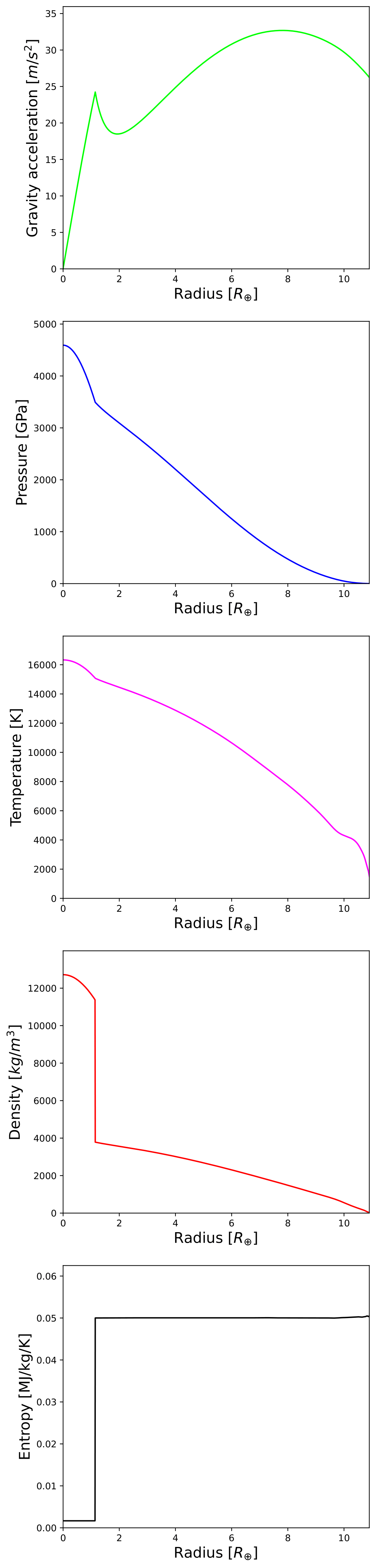
Interior structure profiles for a Jupiter analog with GASTLI.
Additionally, we can show with a circle diagram the size of the core with respect to the size of the planet from the center up to 1000 bar (default interior-atmosphere boundary). For this diagram, the radii at which the core-envelope boundary and the outer envelope interface are located is obtained with the radius profile array (coupling_class_object.myplanet.r), and an array named coupling_class_object.myplanet.intrf, which indicates the indexes of the interior profile arrays that correspond to the interfaces between the different layers. Element i = 1 of this array corresponds to the core-envelope interfaces, while element i = 2 is the outer (surface) boundary of the envelope. Since the indexing follows the Fortran convention, the final Python index is the original index minus 1 (see example below):
# Plot planet core and envelope
fig = plt.figure(figsize=(6, 6))
ax = fig.add_subplot(1, 1, 1)
# Core radius
r_core = my_coupling.myplanet.r[my_coupling.myplanet.intrf[1] - 1]\
      / my_coupling.myplanet.r[my_coupling.myplanet.intrf[2] - 1]
# Interior-atmosphere boundary
r_lm = my_coupling.myplanet.r[my_coupling.myplanet.intrf[2] - 1]\
    / my_coupling.myplanet.r[my_coupling.myplanet.intrf[2] - 1]
# Circles
circle4 = plt.Circle((0.5, 0.5), r_core, color='teal')
circle3 = plt.Circle((0.5, 0.5), r_lm, color='mediumspringgreen')
ax.add_patch(circle3)
ax.add_patch(circle4)
plt.tick_params(axis='both', which='both', bottom=False, top=False, \
             labelbottom=False, right=False, left=False, labelleft=False)
plt.axis('equal')
# Save figure
fig.savefig('core_and_envelope.pdf', bbox_inches='tight', format='pdf', dpi=1000)
plt.close(fig)
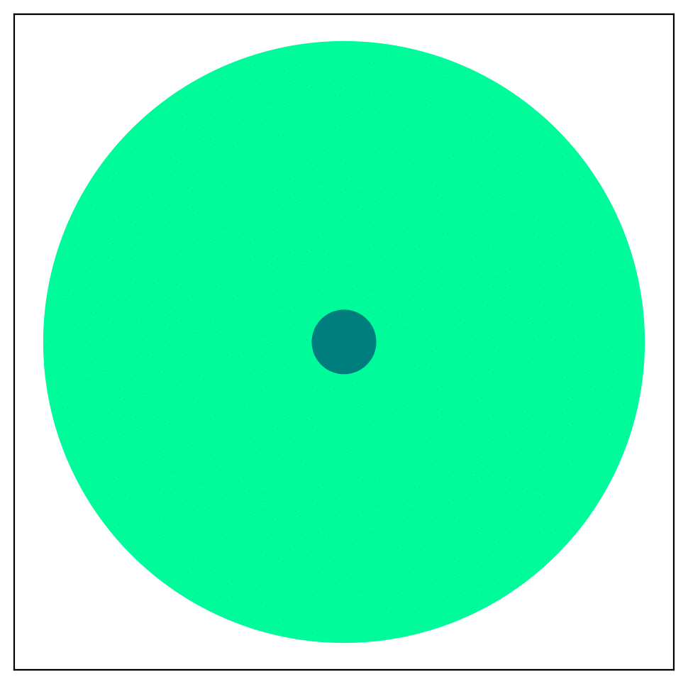
Size of core in comparison to planet size (interior only).
Atmospheric profiles
Similar to the interior structure profiles, the atmospheric profiles can be obtained as:
Gravity in m/s 2:
coupling_class_object.myatmmodel.g_odePressure in Pa:
coupling_class_object.myatmmodel.P_odeTemperature in K:
coupling_class_object.myatmmodel.T_odeDensity in kg/m 3:
coupling_class_object.myatmmodel.rho_odeRadius in m:
coupling_class_object.myatmmodel.r_ode
Following the example above, we can plot the atmospheric profiles as (the coupling class object is still my_coupling):
# Plot atm. profiles
fig = plt.figure(figsize=(24, 6))
# Panel 1: temperature
ax = fig.add_subplot(1, 4, 1)
plt.plot(my_coupling.myatmmodel.T_ode,my_coupling.myatmmodel.P_ode/1e5, '-', color='black')
plt.ylabel(r'Pressure [bar]', fontsize=16)
plt.xlabel(r'Temperature [K]', fontsize=16)
ax.invert_yaxis()
ax.set_yscale('log')
plt.ylim(1e3,2e-2)
# Panel 2: density
ax = fig.add_subplot(1, 4, 2)
plt.plot(my_coupling.myatmmodel.rho_ode,my_coupling.myatmmodel.P_ode/1e5, '-', color='blue')
plt.ylabel(r'Pressure [bar]', fontsize=16)
plt.xlabel(r'Density [kg/m$^{3}$]', fontsize=16)
ax.invert_yaxis()
ax.set_yscale('log')
plt.ylim(1e3,2e-2)
# Panel 3: gravity
ax = fig.add_subplot(1, 4, 3)
plt.plot(my_coupling.myatmmodel.g_ode,my_coupling.myatmmodel.P_ode/1e5, '-', color='orange')
plt.ylabel(r'Pressure [bar]', fontsize=16)
plt.xlabel('Gravity acceleration [m/s$^{2}$]', fontsize=16)
ax.invert_yaxis()
ax.set_yscale('log')
plt.ylim(1e3,2e-2)
# Panel 4: pressure and radius
ax = fig.add_subplot(1, 4, 4)
# Rjup = 7.149e7    # Jupiter radius in m
plt.plot(my_coupling.myatmmodel.r/7.149e7,my_coupling.myatmmodel.P_ode/1e5, '-', color='red')
plt.ylabel(r'Pressure [bar]', fontsize=16)
plt.xlabel('Radius [$R_{Jup}$]', fontsize=16)
ax.invert_yaxis()
ax.set_yscale('log')
plt.ylim(1e3,2e-2)
# Save figure
fig.savefig('atmospheric_profiles.pdf', bbox_inches='tight', format='pdf', dpi=1000)
plt.close(fig)
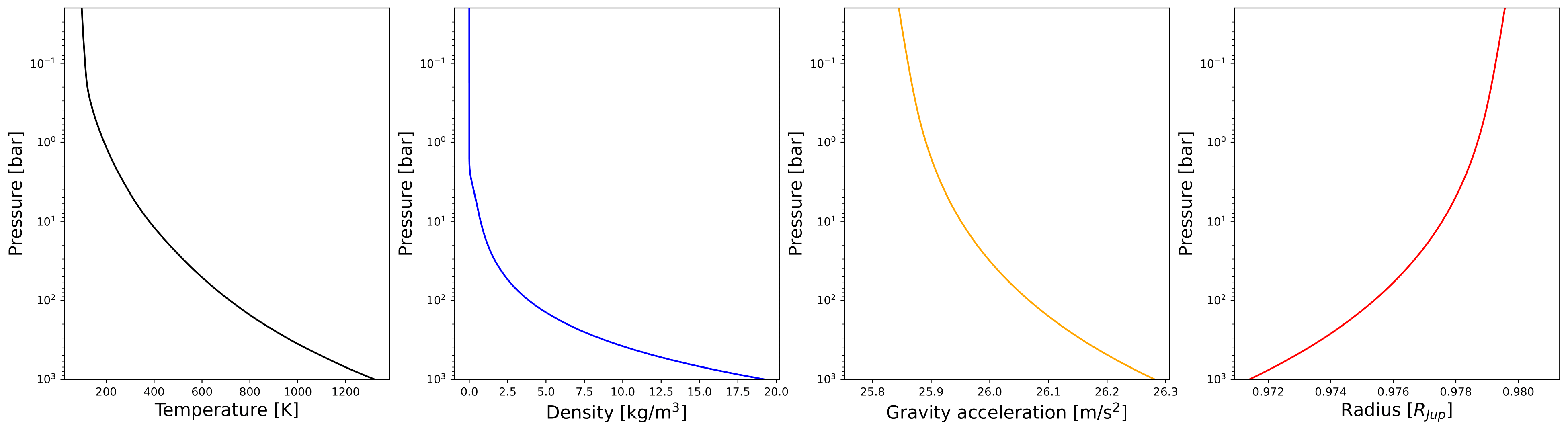
Atmospheric profiles for Jupiter analogue with GASTLI’s default atmospheric grid.
Note
In the following example, we make use of the optional input parameter Rguess. This is the initial guess of the planet radius for the interior-atmosphere algorithm. The default value is Jupiter’s radius (11.2 Earth radii), but for smaller planets (lower mass and/or higher metal content) using a lower value of Rguess than the default speeds convergence.
We can combine the pressure-temperature profile from the interior and the atmosphere to obtain the complete adiabat. We can use the GASTLI class water_curves to overplot the water phase diagram to see if water condensation occurs in the upper layers of the atmosphere:
# Import GASTLI modules
import gastli.water_curves as water_curv
import gastli.Coupling as cpl
# Other modules
from matplotlib import pyplot as plt
import numpy as np
# Cold planet model
my_coupling = cpl.coupling()
# Input for interior
# Mearth units
M_P = 50.
# Internal temperature
Tintpl = 50.
# Equilibrium temperature
Teqpl = 300.
# Core mass fraction
CMF = 0.5
# Envelope log-metallicity is solar
log_FeHpl = 2.4
# C/O ratio is solar
CO_planet = 0.55
# Run coupled interior-atmosphere model
my_coupling.main(M_P, CMF, Teqpl, Tintpl, CO=CO_planet, log_FeH=log_FeHpl,Rguess=6.)
# Hot planet model
my_coupling_hot = cpl.coupling()
my_coupling_hot.main(M_P, CMF, 1000., Tintpl, CO=CO_planet, log_FeH=log_FeHpl,Rguess=6.)
# Water phase diagram class
water_phase_lines = water_curv.water_curves()
# Plot
fig,ax = plt.subplots(nrows=1,ncols=1)
plt.title(r'M = 50 $M_{\oplus}$, CMF = 0.5, $T_{int}$ = 50 K, [Fe/H] = 250 x solar')
water_phase_lines.plot_water_curves(ax)
plt.plot(my_coupling.myplanet.T, my_coupling.myplanet.P, '-', color='blue',label=r'$T_{eq}$ = 300 K')
plt.plot(my_coupling.myatmmodel.T_ode, my_coupling.myatmmodel.P_ode, '-', color='blue')
plt.plot(my_coupling_hot.myplanet.T, my_coupling_hot.myplanet.P, '-', color='red',label='$T_{eq}$ = 1000 K')
plt.plot(my_coupling_hot.myatmmodel.T_ode, my_coupling_hot.myatmmodel.P_ode, '-', color='red')
plt.yscale('log')
plt.xscale('log')
plt.ylabel(r'Pressure [Pa]', fontsize=14)
plt.xlabel(r'Temperature [K]',fontsize=14)
xmin = 100
xmax = 2e4
plt.xlim((xmin,xmax))
plt.ylim((1,1e15))
plt.text(1000, 1e9, 'Supercritical')
plt.text(400, 5e10, 'Ice VII')
plt.text(300, 5e7, 'Liquid')
plt.text(1000, 100, 'Vapor')
plt.legend()
# Save figure
fig.savefig('phase_diagram.pdf',bbox_inches='tight',format='pdf', dpi=1000)
plt.close(fig)
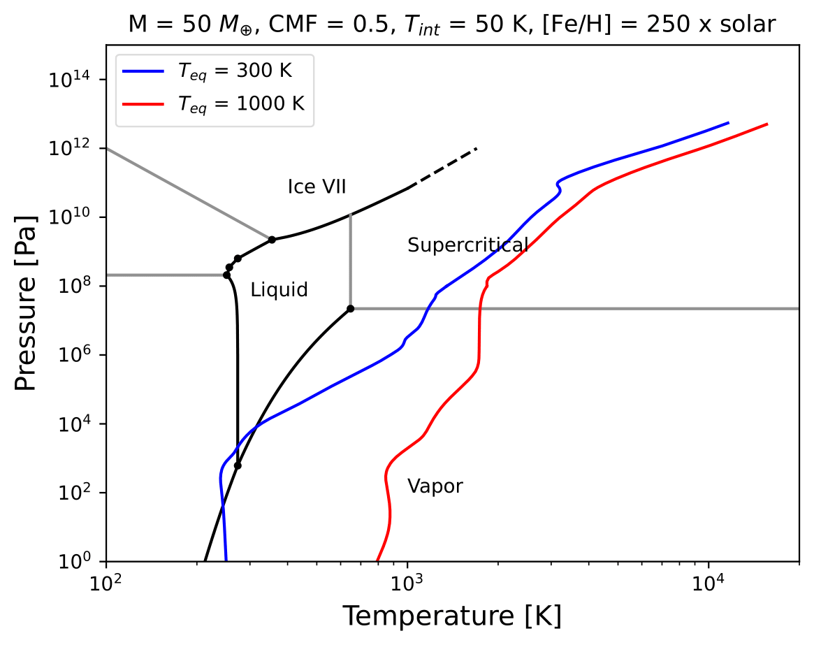
Pressure-temperature adiabats for a metal-rich planet at low (300 K) and high irradiation (1000 K). Water condenses in the upper layers of the atmosphere in the cold planet case.
Mass-radius diagram
To generate a mass-radius curve, you need to call the coupling class several times, and modify the mass in each call. A for loop can do this:
# Import coupling module
import gastli.Coupling as cpl
# Other Python modules
import numpy as np
# Input for interior
## 1 Mjup in Mearth units
Mjup = 318.
mass_array = Mjup * np.arange(0.05,1.6,0.05)
n_mrel = len(mass_array)
## Internal temperature
Tintpl = 107.     # K
## Equilibrium temperature
Tstar = 5777.     # K
Rstar = 0.00465   # AU
ad = 5.2          # AU
Teq_4 = Tstar**4./4. * (Rstar/ad)**2.
Teqpl = Teq_4**0.25
# Core mass fraction
CMF = 0.
# Mass-radius curve output file
file_out = open('Jupiter_MRrel_CMF0_logFeH_0.dat','w')
file_out.write('  M_int[M_E]  M_tot[M_E]  x_core  ')
file_out.write('T_surf[K]  R_bulk[R_J]  R_tot[R_J]  T_int[K]  Zenv  z_atm[R_J] ')
file_out.write("\n")
# For loop that changes the mass in each call of the coupling class
for k in range(0, n_mrel):
    M_P_model = mass_array[k]
    print('---------------')
    print('Mass [Mearth] = ', M_P_model)
    print('Model = ', k+1, ' out of ', n_mrel)
    print('---------------')
    # Create coupling class (this also resets parameters)
    my_coupling = cpl.coupling(pow_law_formass=0.31)
    # Case 1, log(Fe/H) is known
    # You must have FeH_flag=True, which is the default value
    my_coupling.main(M_P_model, CMF, Teqpl, Tintpl, CO=0.55, log_FeH=0.)
    # Save data
    file_out.write('%s %s' % ("  ", str(M_P_model)))
    file_out.write('%s %s' % ("  ", str(my_coupling.Mtot)))
    file_out.write('%s %s' % ("  ", str(CMF)))
    file_out.write('%s %s' % ("  ", str(my_coupling.T_surf)))
    file_out.write('%s %s' % ("  ", str(my_coupling.Rbulk_Rjup)))
    file_out.write('%s %s' % ("  ", str(my_coupling.Rtot)))
    file_out.write('%s %s' % ("  ", str(Tintpl)))
    file_out.write('%s %s' % ("  ", str(my_coupling.myatmmodel.Zenv_pl)))
    zatm_RJ = my_coupling.Rtot - my_coupling.Rbulk_Rjup
    file_out.write('%s %s' % ("  ", str(zatm_RJ)))
    file_out.write("\n")
    file_out.flush()
# End of for loops
file_out.close()
We can then read the file and plot the mass-radius curve. In this file, the columns M_tot[M_E] and R_tot[R_J] are the total mass and radius in Earth masses and Jupiter radii units, respectively. We can plot them as:
# Import modules
import matplotlib.pyplot as plt
import numpy as np
import pandas as pd
# Read data from file
data = pd.read_csv('Jupiter_MRrel_CMF0_logFeH_0.dat', sep='\s+',header=0)
M_CMF0_logFeH0_Tint107 = data['M_tot[M_E]']
R_CMF0_logFeH0_Tint107 = data['R_tot[R_J]']
# Mass-radius plot
xmin = 0.04
xmax = 1.50
ymin = 0.78
ymax = 1.05
Mjup = 318.
fig = plt.figure(figsize=(6,6))
ax = fig.add_subplot(1, 1, 1)
ax.tick_params(axis='both', which='major', labelsize=14)
plt.title("GASTLI, solar envelope composition")
plt.plot(M_CMF0_logFeH0_Tint107/Mjup, R_CMF0_logFeH0_Tint107, color='black',linestyle='solid',\
      linewidth=4, label=r'CMF = 0')
# Jupiter ref
plt.plot([1.], [1.], 'X', color='darkorange',label=r'Jupiter',markersize=14,\
      markeredgecolor='black')
plt.xlim((xmin,xmax))
plt.ylim((ymin,ymax))
plt.xlabel(r'Mass [$M_{Jup}$]',fontsize=14)
plt.ylabel(r'Radius [$R_{Jup}$]',fontsize=14)
plt.legend()
fig.savefig('Jupiter_MRrel.pdf',bbox_inches='tight',format='pdf', dpi=1000)
plt.close(fig)
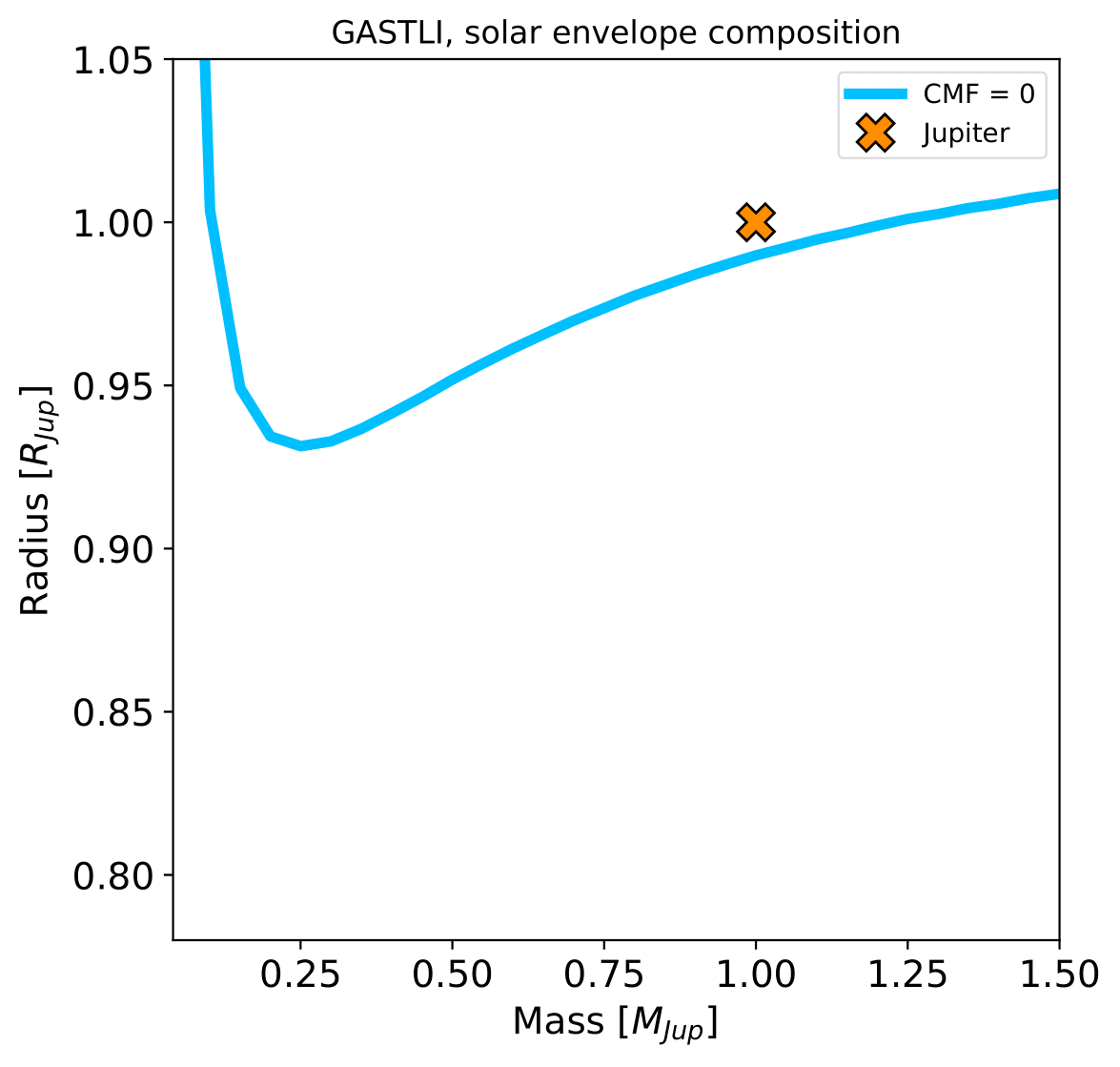
Mass-radius curve for a Jupiter analogue with a homogeneous, solar composition (CMF = 0, log(Fe/H) = 0).